Detector banks, pindex joins, and real PID

The pid in REC::Particle is a starting point, not the truth. A real electron ID checks the detector response: did it deposit the right fraction of its energy in the calorimeter, and did it fire the Cherenkov? That information lives in REC::Calorimeter and REC::Cherenkov, linked to particles by pindex. Learning to join on pindex is the single most useful CLAS12-specific skill.

The join, for one particle

The trigger electron is REC::Particle row 0, so its detector rows are the ones with pindex == 0. To get its total calorimeter energy, filter and sum:

cal = f.arrays("REC::Calorimeter", ["pindex", "layer", "energy"])

e_ecal = ak.sum(cal.energy[cal.pindex == 0], axis=1)     # total ECAL energy, per event

cal.energy[cal.pindex == 0] keeps, in each event, only the calorimeter rows pointing at particle 0; ak.sum(..., axis=1) adds them up per event. That's the whole pattern.

Sampling fraction — an electron's signature

A CLAS12 calorimeter is a sampling calorimeter: an electron deposits a roughly constant fraction — about 0.25 — of its momentum, independent of energy. Hadrons deposit far less. So $E_{\text{cal}}/p$ is a powerful electron/pion separator:

p3e = np.sqrt(p[:, 0].px**2 + p[:, 0].py**2 + p[:, 0].pz**2)   # electron |p|
sf  = ak.to_numpy(e_ecal) / ak.to_numpy(p3e)                   # sampling fraction

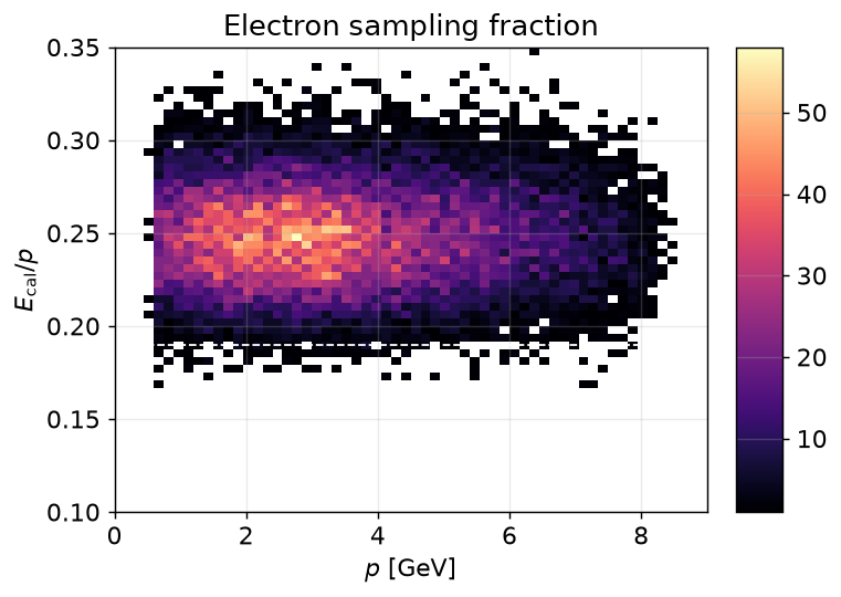
The band sits flat at $\langle E_{\text{cal}}/p\rangle \approx 0.248$ (σ ≈ 0.025) across all momenta — exactly the electron signature. The pion contamination would sit far lower, near the MIP floor. The dashed line at 0.19 is a simple cut; real analyses use a momentum-dependent $\mu(p) \pm N\sigma(p)$ band, because the resolution widens at low $p$.

good_sf = sf > 0.19               # first-order electron calorimeter cut

You can also break the deposit down by layer — PCAL is layer == 1, ECIN 4, ECOUT 7 — which powers more refined cuts (e.g. a minimum PCAL energy):

pcal = ak.sum(cal.energy[(cal.pindex == 0) & (cal.layer == 1)], axis=1)

Beyond particle 0

Every mask above is written for pindex == 0 — the trigger electron. That is the right way to learn the join, and the wrong way to scale it: a hadron analysis needs the same quantity for every particle, and there is no pindex == i to loop over cheaply.

ox.group_by_index does the join for all of them at once, regrouping the bank so each particle owns its rows:

part = f.arrays("REC::Particle", ["pid", "px", "py", "pz"])
by   = ox.group_by_index(cal, ak.num(part))          # events * particles * var * {...}

part["cal_energy"] = ak.sum(by.energy, axis=-1)      # per particle, not per event
part["pcal"]       = ak.sum(by[by.layer == 1].energy, axis=-1)

cal_energy is now a column beside px, so cuts and plots treat it like any other. ox.link goes further and wires both directions across a whole multi-bank read — see joining detector banks by pindex.

Cherenkov — the other half

The HTCC fires for electrons (and fast pions above ~4.9 GeV). Its photoelectron count nphe cleanly tags electrons:

ch = f.arrays("REC::Cherenkov", ["pindex", "nphe"])
e_nphe = ak.sum(ch.nphe[ch.pindex == 0], axis=1)      # ~13 for electrons here
good_htcc = e_nphe > 2                                 # standard nphe > 2 cut

The join, for every particle

Sometimes you need detector info for particles that aren't row 0 — every photon's cluster energy, say. The general "attach a per-particle sum" join broadcasts each particle's index against every detector row's pindex:

part_idx = ak.local_index(p.pid, axis=1)              # 0,1,2,… within each event

# pair every particle with every cal row (grouped by particle), keep the matches
idx, cpid = ak.unzip(ak.cartesian([part_idx, cal.pindex], axis=1, nested=True))
_,   cE   = ak.unzip(ak.cartesian([part_idx, cal.energy], axis=1, nested=True))
ecal_per_particle = ak.sum(ak.where(idx == cpid, cE, 0.0), axis=2)

Now ecal_per_particle has the same jagged shape as p.pid: one calorimeter-energy sum per particle. ecal_per_particle[:, 0] reproduces the electron result exactly. For a single selected particle the filter form is simpler and faster; reach for this broadcast form when you genuinely need all particles at once.

Building an electron ID

Stack the cuts into one boolean, and count what each one costs — a cutflow is how you debug a selection:

n0 = len(sf)
cutflow = {
    "trigger e⁻":   n0,
    "+ SF > 0.19":  int(ak.sum(good_sf)),
    "+ nphe > 2":   int(ak.sum(good_sf & good_htcc)),
    "+ |vz| < 10":  int(ak.sum(good_sf & good_htcc & (np.abs(p[:, 0].vz) < 10))),
}

On real data you'd add chi2pid (the timing consistency), a vertex cut (the target is a few cm long — -8 < vz < 2 for RG-A), and sector-dependent details. The point is the pattern: express each cut as an aligned boolean mask, & them, and track the survivors.

Fiducial cuts

Detectors have edges and dead zones where reconstruction is unreliable. Fiducial cuts remove particles too close to them. The calorimeter ones use the cluster's position in detector coordinates (lu, lv, lw — distances from the PCAL edges):

cal = f.arrays("REC::Calorimeter", ["pindex", "layer", "lv", "lw"])
# electron's PCAL cluster position:
e_pcal = cal[(cal.pindex == 0) & (cal.layer == 1)]
lv = ak.firsts(e_pcal.lv)
lw = ak.firsts(e_pcal.lw)
fiducial = (lv > 9) & (lw > 9)              # drop clusters within 9 cm of an edge

The drift-chamber fiducial cuts (from REC::Traj, the trajectory bank) remove tracks near the DC sector boundaries and are torus-polarity dependent. They're not in this sample's banks, but the mechanic is identical: read the bank, join on pindex, cut on a geometric variable.

Corrections — where they go

Reconstructed momenta aren't perfect: charged particles lose energy in material (energy-loss corrections) and the tracking has small biases (momentum corrections). CLAS12 provides these as functions of $(p, \theta, \phi, \text{sector}, \text{torus})$ per run period.

They slot in as a step that produces corrected columns before you do kinematics:

def correct_momentum(part, torus):
    # ILLUSTRATIVE placeholder — real coefficients come from the collaboration
    # (e.g. clas12-analysis momentum-correction packages), keyed to your run period.
    scale = 1.0 + 0.0            # replace with the real p,θ,φ,sector function
    return ak.zip({"px": part.px * scale, "py": part.py * scale, "pz": part.pz * scale})

Two honest notes: (1) the coefficients are collaboration-specific and period-specific — don't hardcode someone else's; (2) apply corrections before computing $Q^2$, invariant masses, etc., and once you've settled them you can persist the corrected columns with update so downstream jobs skip the recomputation.

With clean particles and honest kinematics, we can go after exclusive final states.

Exclusive channels →