Reconstructing particles: invariant & missing mass

Inclusive DIS only used the electron. Real analyses combine particles: pair two photons into a $\pi^0$, add a hadron for SIDIS, or reconstruct an exclusive reaction by what's missing. This is where Awkward's combinatorics earn their keep.

$\pi^0 \to \gamma\gamma$: invariant mass

A $\pi^0$ decays to two photons before it reaches the detector, so you never see it directly — you see two photons and reconstruct their invariant mass. If a pair came from a $\pi^0$, that mass equals $m_{\pi^0} = 0.135$ GeV.

The move is ak.combinations, which forms all unordered pairs within each event:

photons = p[p.pid == 22]
pairs = ak.combinations(photons, 2)      # every γγ pair, per event
g1, g2 = ak.unzip(pairs)                  # two aligned photon arrays

def inv_mass_2(a, b):                      # photons are massless: E = |p|
    Ea = np.sqrt(a.px**2 + a.py**2 + a.pz**2)
    Eb = np.sqrt(b.px**2 + b.py**2 + b.pz**2)
    return np.sqrt(np.maximum(0, (Ea + Eb)**2
                   - (a.px + b.px)**2 - (a.py + b.py)**2 - (a.pz + b.pz)**2))

m_gg = ak.flatten(inv_mass_2(g1, g2))      # all pair masses, flattened

import mplhep as hep

counts, edges = np.histogram(ak.to_numpy(m_gg), bins=80, range=(0.05, 0.35))
hep.histplot(counts, edges, histtype="fill", alpha=0.85)

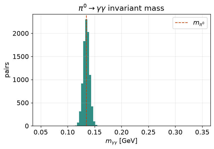
A clean peak at 0.135 GeV (σ ≈ 6 MeV here; ~10–15 MeV on real data, set by the calorimeter resolution) over a combinatorial background. To use the $\pi^0$s — count them, or feed them into a higher final state — cut a window and treat each surviving pair as a $\pi^0$ candidate:

is_pi0 = (m_gg > 0.11) & (m_gg < 0.16)

On real data you'd fit the peak (a Gaussian plus a polynomial background) and sideband-subtract, but the window is the first cut.

Combinatorial background

With three photons in an event, ak.combinations gives three pairs and at most one is a true $\pi^0$ — the rest are the background under the peak. This is intrinsic to combinatorics, not a bug; sideband subtraction is how you remove it.

Semi-inclusive DIS: adding a hadron

SIDIS detects the scattered electron and a hadron, and describes the hadron in variables relative to the virtual photon $q = k - k'$:

• $z = E_h/\nu$ — the fraction of the energy transfer the hadron carries,
• $p_T$ — the hadron momentum transverse to $\vec q$,
• $\phi_h$ — the azimuth of the hadron around $\vec q$ (the Trento angle).

M_PIP = ox.pdg_mass(211)     # 0.13957039 GeV
pip = p[p.pid == 211]
lead = ak.argmax(np.sqrt(pip.px**2 + pip.py**2 + pip.pz**2), axis=1, keepdims=True)
h = ak.firsts(pip[lead])          # leading π⁺ per event (None if the event has none)

Eh = np.sqrt(h.px**2 + h.py**2 + h.pz**2 + M_PIP**2)
z  = Eh / kin.nu                  # kin.nu from the DIS kinematics function

# q vector = beam - scattered electron
qx, qy, qz = -ele.px, -ele.py, 10.604 - ele.pz
qmag = np.sqrt(qx**2 + qy**2 + qz**2)
h_par = (h.px*qx + h.py*qy + h.pz*qz) / qmag          # momentum along q
pT = np.sqrt(np.maximum(0, h.px**2 + h.py**2 + h.pz**2 - h_par**2))

z runs 0–1 (mean ≈ 0.5 on the sample) and pT up to ~1–2 GeV — the SIDIS kinematic plane. The Trento $\phi_h$ needs the cross products of the lepton and hadron planes; scikit-hep vector makes that a one-liner (q.deltaphi(h) after rotating into the $\vec q$ frame), which is the point at which a four-vector library stops being optional.

Exclusive reactions: missing mass

The most powerful trick: if you detect all but one particle in a reaction, the undetected particle's mass is the missing mass — and it peaks at that particle's true mass. For $ep \to e'\pi^+ n$, detecting $e'$ and $\pi^+$ and missing the neutron:

$$M_X^2 = \big(k + p_{\text{target}} - k' - p_{\pi}\big)^2 \;\xrightarrow{\ ep\to e'\pi^+ n\ }\; m_n^2$$

M_P = ox.pdg_mass(2212)
beam_E, target_E = 10.604, M_P                    # target proton at rest

miss_E  = beam_E + target_E - Ee_scattered - Eh   # Ee_scattered = |p| of e'
miss_px = -(ele.px + h.px)
miss_py = -(ele.py + h.py)
miss_pz = beam_E - (ele.pz + h.pz)
MX = np.sqrt(np.maximum(0, miss_E**2 - miss_px**2 - miss_py**2 - miss_pz**2))

counts, edges = np.histogram(ak.to_numpy(MX[~ak.is_none(MX)]), bins=80, range=(0.5, 2.0))
hep.histplot(counts, edges, histtype="fill", alpha=0.85)

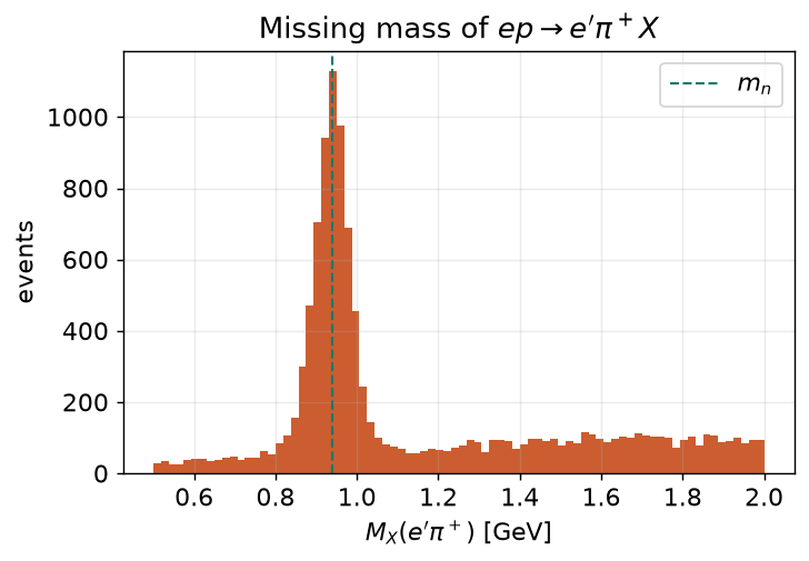
The sharp peak at the neutron mass (0.94 GeV) is the exclusive $ep\to e'\pi^+ n$ signal; the broad continuum above it is SIDIS, where extra undetected particles push the missing mass up. Isolate the exclusive channel with a missing-mass cut:

exclusive = (MX > 0.85) & (MX < 1.03)      # a window around the neutron

That's the whole idea behind exclusive physics at CLAS12 — DVCS ($ep\to e'p\gamma$), $\pi^0$ electroproduction, and the rest are the same recipe with more detected particles and tighter missing-mass (or missing-momentum) constraints.

Putting it together

A realistic selection chains everything you've built: trigger-electron ID (sampling fraction + Cherenkov + vertex + fiducial), DIS cuts ($Q^2$, $W$, $y$), a hadron with its own PID, and a missing-mass or invariant-mass window — each an aligned boolean mask, &-ed together, with a cutflow tracking the survivors. That analysis object is what you then want to run over all the data, fast.

Scaling up →