Inclusive DIS kinematics

With a scattered electron in hand, you can compute the deep-inelastic scattering variables — the coordinates every CLAS12 analysis lives in. This is the canonical first physics result.

The setup

An electron of energy $E$ scatters off a proton at rest, emerging with energy $E'$ at angle $\theta$. The virtual photon exchanged carries four-momentum $q = k - k'$ (beam minus scattered electron). From it:

$$Q^2 = -q^2 = 4EE'\sin^2\!\tfrac{\theta}{2}, \quad \nu = E - E', \quad x_B = \frac{Q^2}{2M\nu}, \quad y = \frac{\nu}{E}, \quad W = \sqrt{M^2 + 2M\nu - Q^2}$$

$Q^2$ is the resolving power (virtuality), $\nu$ the energy transfer, $x_B$ the Bjorken scaling variable (loosely, the struck quark's momentum fraction), $y$ the inelasticity, and $W$ the invariant mass of everything except the scattered electron — the hadronic final state. "Deep inelastic" means $Q^2 \gtrsim 1$ GeV² and $W > 2$ GeV (above the resonance region).

Beam energy is yours to supply

It is not in the file. Set it from the run period. Here it's 10.604 GeV (RG-A). Get this wrong and every number on this page is wrong.

The code

import numpy as np
import awkward as ak

BEAM = 10.604          # GeV — from the run period, NOT the file
M_P  = ox.pdg_mass(2212)   # proton mass in GeV

# `ele` is the scattered electron from the previous page (one record per event).
Ee    = np.sqrt(ele.px**2 + ele.py**2 + ele.pz**2)     # E' ≈ |p| (electron is ~massless)
theta = np.arccos(ele.pz / Ee)

Q2 = 4 * BEAM * Ee * np.sin(theta / 2)**2
nu = BEAM - Ee
xB = Q2 / (2 * M_P * nu)
y  = nu / BEAM
W  = np.sqrt(M_P**2 + 2 * M_P * nu - Q2)

Every one of these is a plain per-event array — no loop, no four-vector class. Q2[i], W[i], … are event $i$'s kinematics.

The DIS cut

Restrict to the deep-inelastic region and drop unphysical tails:

dis = (Q2 > 1.0) & (W > 2.0) & (y > 0.0) & (y < 0.85)
Q2, xB, W = Q2[dis], xB[dis], W[dis]

The y < 0.85 cut removes the region where radiative effects and the falling cross-section make electrons unreliable — a standard CLAS12 choice.

Look at it

import matplotlib.pyplot as plt
import mplhep as hep          # histogram helpers — we never call hep.style.use()

# bin first, then draw: hep.hist2dplot takes counts + edges
H, xe, ye = np.histogram2d(ak.to_numpy(xB), ak.to_numpy(Q2),
                           bins=(60, 60), range=((0, 0.8), (0, 8)))
H = np.where(H == 0, np.nan, H)          # leave empty bins blank

fig, ax = plt.subplots()
hep.hist2dplot(H, xe, ye, ax=ax, cmap="viridis")     # colorbar included
ax.set(xlabel="$x_B$", ylabel="$Q^2$ [GeV$^2$]")

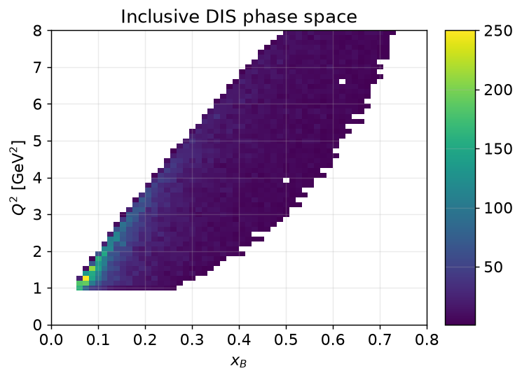
The diagonal band is the hallmark DIS correlation: at fixed beam energy, $Q^2$ and $x_B$ are kinematically tied ($Q^2 = x_B\, y\, s$, with $s = 2ME + M^2$), and the detector's angular acceptance carves out the populated region. On the sample, $Q^2$ runs from 1 to ~11 GeV² (mean ≈ 3.8) and:

W = ...                       # as above, before the W cut
counts, edges = np.histogram(ak.to_numpy(W), bins=70, range=(2, 4.5))
hep.histplot(counts, edges, histtype="fill", alpha=0.85)

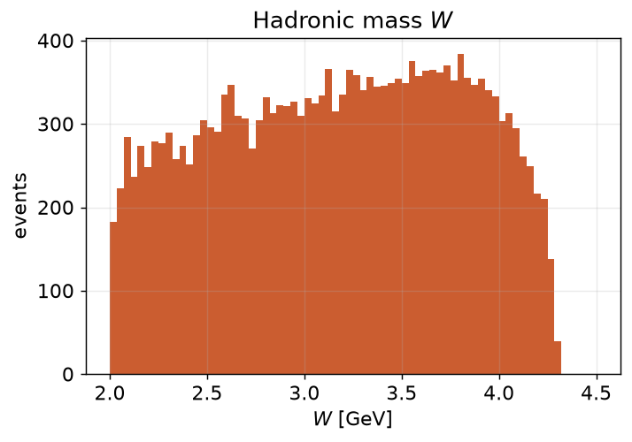
On real data this same plot shows sharp resonance peaks below $W = 2$ GeV (the $\Delta(1232)$ and friends) that the synthetic sample doesn't model — which is exactly why the $W > 2$ cut defines "deep inelastic." Seeing those peaks appear when you run this on a real DST is a good sanity check that your electron selection and beam energy are right.

A reusable kinematics function

You'll want these variables on every event, so package them:

def dis_kinematics(ele, beam=10.604, target_mass=M_P):
    Ee    = np.sqrt(ele.px**2 + ele.py**2 + ele.pz**2)
    theta = np.arccos(ele.pz / Ee)
    Q2 = 4 * beam * Ee * np.sin(theta / 2)**2
    nu = beam - Ee
    return ak.zip({
        "Q2": Q2, "nu": nu, "xB": Q2 / (2 * target_mass * nu),
        "y": nu / beam, "W": np.sqrt(target_mass**2 + 2 * target_mass * nu - Q2),
    })

kin = dis_kinematics(ele)
kin.Q2, kin.W, kin.xB      # fields on one per-event record

ak.zip bundles the arrays into a record so kin travels as a unit and stays aligned with ele. We'll extend this with hadron variables in Exclusive channels.

Next, the detector banks — where PID gets serious.

Detector banks & PID →